Constructing binary trees using relative branch encoding

Structured depth-first search

Let’s start with that last idea. We take the basic recursive depth-first search algorithm and extend the return value to include the attachment point of the node value returned. We’ll assign the furthest-right locus 0 and number up from there. This means adding a 1 for every time we recurse and explore a left branch.

The generator below yields tuples with an absolute branch location and the value at that location, in pre-order sequence:

def dfs_structural(node: Node, branch_id: int = 0) -> Iterator[Tuple[int, Any]]:
    if node is not None:
        yield branch_id, node.value
        yield from dfs_structural(node.left, branch_id=branch_id + 1)
        yield from dfs_structural(node.right, branch_id=branch_id)

While this does a little bit more work than the typical depth-first search algorithm, it shares its time and memory complexities of linear and height-dependent respectively.

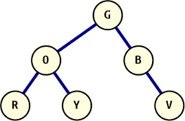
A binary tree with text values.

This binary tree is sorted, but that only becomes obvious once you learn that the letters refer to the colors of the rainbow, at which point its chromatic ordering becomes clear.

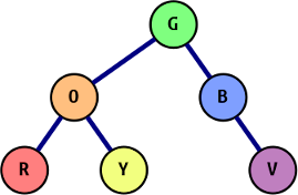
The same tree as above, now colored to illustrate the chromatic ordering.

Given the binary tree pictured on the right, the output of our function captured into a list looks like this: [(0, "G"), (1, "O"), (2, "R"), (1, "Y"), (0, "B"), (0, "V")]. This uses the same numbering scheme from the last post, but for completeness, the tree is described in the following way:

1. (0, "G") places the root, green, in the only available starting location of the tree; from here, the left and right children are explored in sequence:
2. (1, "O") places orange on branch 1 as left child of the root and the search recurses down to this node;
3. (2, "R") places red on the number 2 branch, left of the previous node. Each subsequent left branch exploration has a higher branch-id, because in branching left, attachment loci are created on the path up to the root;
4. (1, "Y") the red node (which provides branch-ids 2 and 3) has no children, so recursion ends there. After that, execution of the orange node’s traversal continues and extends to its right child, which is where we find yellow on branch 1.
5. (0, "B") another continuation of recursion, this time back to the root, where blue attaches on the right side. This step to the right from the root makes this node the new zero node in the tree when it comes to branch numbering: there are no open branches on any node above this one;
6. (0, "V") finally attaches violet to the right of blue, again without a change of branch-id, and a shift of the zero node.

Relative branch encoding

While the output from the previous function is enough to rebuild the original tree, it doesn’t quite focus on the ease of reconstruction, or the brevity of the communication, which is one of the reasons we started this.

So, before we send this sequentialisation over the wire, there are a number of small tweaks we’ll make:

1. Change the stream of 2-tuples to a flat stream of values and branch offsets. We trade homogeneous output (2-tuples of branch id and node value) for a reduction of two characters for each tree element. Iteration doesn’t become any harder (shown later) and it allows a minor other optimisation:
2. Now that we don’t need matched pairs, drop the attachment location of the root node, since there is no actual choice in where to place that;
3. Change the absolute branch_id to a relative one: 0 for a left child, 1 for a right child and 2 and up to indicate right children after backtracking (and so we still get our numbering to start from the left).

def dfs_relative(root):
    def _relative_traverser(traversal):
        last_branch_id = 0
        for branch_id, value in traversal:
            delta, last_branch_id = 1 + last_branch_id - branch_id, branch_id
            yield delta
            yield value

    return islice(_relative_traverser(dfs_structural(root)), 1, None)

The inner function takes the iterator returned by dfs_structural and turns it into a relative one by tracking the difference between the current and last branch_id, turning the absolute values into just the changes. Instead of returning tuples it returns the delta and node value in sequence.

The final statement reads a bit terse, but it returns the absolute-to-relative conversion of the traversal, skipping the first value from the resulting iterator. When captured into a list, our tree from before is now represented as ["G", 0, "O", 0, "R", 2, "Y", 2, "B", 1, "V"].

Tree reconstruction

Constructing a tree from this stream is pretty straightforward, the only “trick” we need is a pairwise iterator, which is easily achieved by taking a single iterator from the pre-order sequence and zipping it on itself:

def tree_reconstruct(structural_preorder):
    ivalues = iter(structural_preorder)
    root = node = Node(next(ivalues))
    stack = []
    for branch_id, value in zip(ivalues, ivalues):
        if branch_id == 0:
            stack.append(node)
            node.left = node = Node(value)
        else:
            for _ in range(1, branch_id):
                node = stack.pop()
            node.right = node = Node(value)
    return root

Like our previous iterative functions that operate on or create a tree, we maintain a small stack to account for backtracking. If the relative position is 0 we attach it on the left. In other cases we backtrack 0 or more steps (note that range(1, 1) is an empty range) and then attach on the right. Once all values have been processed, the construction is done and the root is returned.

The series of trees below provide a visualisation of the construction process. Each graph shows the tree at the start of a loop iteration, before inserting the next node. Each possible attachment locus is indicated with a number, according to the relative branch numbering scheme.

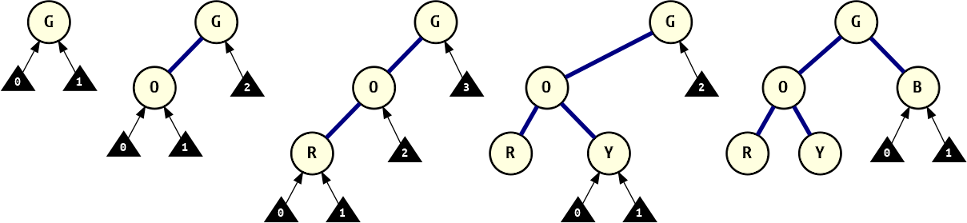
The tree construction process.

Given the sequence ["G", 0, "O", 0, "R", 2, "Y", 2, "B", 1, "V"], this visualises the attachment loci after each ndoe attachment, building up the tree one node at a time.

So, did it work?

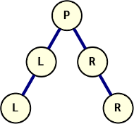
A tree with non-distinct elements, created from its uniquely identifying sequence

One of the goals we set out with was to have a minimal serialised size for something like a JSON transport of a tree. Given some smaller trees consisting of 8-character words, the space savings amount to roughly 40%, though this depends greatly on the length of the values. Worst case we achieve parity (minus a handful of bytes).

What about compression though, how much will that affect the results? A little bit but not a whole lot. Serialising a 1000-node, mostly balanced, tree, where each node contains an 8-character word as its value, the following results are achieved:

• JSON with pre-order and in-order sequences
  • plaintext: 22.026 bytes
  • gzipped: 7.638 bytes (2.9x compression ratio)
• JSON with relative branch-encoded sequence
  • plaintext: 13.012 bytes (41% smaller)
  • gzipped: 5.663 bytes (2.3x compression ratio, still 25% smaller)

Another significant benefit over the dual-sequence method of construction is that with this method, the tree is not restricted to distinct values. Because the structural information is encoded in the sequence and provides complete information for node placement, repeated values do not create ambiguity in the reconstructed tree. The graph on the right shows the tree constructed from ["P", 0, "L", 0, "L", 3, "R", 1, "R"]. Attempting to construct this tree from in-order and pre-order sequences would have four equally possible outcomes without a way to determine the correct one. The algorithm from the first post would place the second L on the right of the first, for example.