Between work, play and other side projects, I’ve been playing around with binary trees. They’re a hugely useful data structure in many fields, but more relevantly in this case, they lend themselves to all sorts of noodling and tinkering. Among the many possible questions is the seemingly simple “how do you serialise a tree?” for inter-process communication, a web-based API or just for the hell of it. And given such a serialisation, how do you reconstruct the original tree from it?
One way is to express each node as a list of three elements: the value of the node, its left child and its right child. Each of these children is its own three-element list (or some form of empty value) and on and on it goes. The end of this serialisation will have a particular signature: ]]]]]]]. Something we have seen before.
I have nothing against brackets per se, but as some have said: “flat is better than nested.” [1] And there are wonderfully flat ways of describing binary trees. This article will cover one such way of representing as, and then constructing a binary tree from a pair of lists, without the need for additional structural information.
Depth-first search
But before we dive into the construction of trees proper, we have to briefly cover how to serialise one. A favourite among interviewers, and elegant as a recursive algorithm, depth-first search is the easiest way of traversing all the nodes in a tree, and extracting their values along the way.
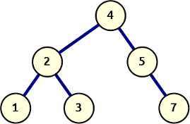
A simple binary search tree
Starting from the root of the tree, the algorithm visits each node by first visiting the left child and recursing there. After that has completed, the right child is visited, again recursing there. This corecursion creates a path that travels down along a left edge, methodically jumps back to the closest unexplored right branch, and repeats that process until all nodes have been covered.
The algorithm avoids costly comparisons, needing only simple equality checks to establish there is a child node to descend to, and the memory use is linear with the height of the tree. In the absolute worst case, this height is equal to the number of nodes in the tree (every child is either a left or right child), but as the tree becomes more balanced, the height approaches O(log n), and so does the memory requirement.
While traversing along this path, the visited nodes (or their values, depending on the requirements) are returned. For a left-to-right traversing algorithm, there are three different options here:
- in-order: yields from the left child, the node itself, and then from the right child; for a binary search tree, this will return the nodes in ascending order;
- pre-order: yields the node itself, from the left child, and then the right child; this describes the visit order of the nodes, also known as topological sorting;
- post-order: yields from the left child, from the right child, and then the node itself. For expression trees this yields a reverse polish notation, which is then easily evaluated using a small stack. [2]
To keep things simple, we’ll keep to the in-order and pre-order traversals, and run them on a simple binary search tree, as detailed below:
from __future__ import annotations
from dataclasses import dataclass
from typing import Any, Optional

@dataclass
class Node:
    value: Any
    left: Optional[Node] = None
    right: Optional[Node] = None

def in_order(node):
    if node is not None:
        yield from in_order(node.left)
        yield node.value
        yield from in_order(node.right)

def pre_order(node):
    if node is not None:
        yield node.value
        yield from pre_order(node.left)
        yield from pre_order(node.right)
It should be evident from the code that the time complexity of these functions is linear with the number of nodes in the tree. Each recursion yields a single node, or does nothing if it’s past the leaf node. Of that latter type, there are exactly n+1 instances, which puts the total number of operations at 2n, asymptotically O(n).
The result of in_order is a generator which yields the values of the tree in left-to-right order. Captured into a list this looks like [1, 2, 3, 4, 5, 7]. By contrast, pre_order will return the nodes in visit-order, which results in a sequence like this: [4, 2, 1, 3, 5, 7].
Construction from pre-order only
No one sequentialisation according to pre-, in- or post-order describes the underlying tree uniquely. Given a tree with distinct elements, either pre-order or post-order paired with in-order is sufficient to describe the tree uniquely.
—Wikipedia, tree traversal
This seems like a pretty bold statement when we look at the pre-order sequence we generated for the example binary search tree. It’s pretty feasible to create an algorithm for that to reconstruct the tree, assuming of course it only has distinct elements (if that’s not the case, unambiguous reconstruction without structural information is impossible).
Remember that a pre-order sequentialisation has the nodes in visit order, so we can create an algorithm to attach each next node to the tree as we construct it. We’ll have to do some back-tracking (following the behavior from the depth-first search algorithm), for which we’ll keep a stack:
- Setup: Create an empty stack and set up the tree’s root
- Take the first value from the pre-order sequentialisation, this is the root
- Create a node from this and push it on the stack
- Store it as both the root and current node
- Loop: Take the next value and compare it to the current node’s value
- smaller: Descent down along the left edge
- Create a new node from this value and push it on the stack
- Set it as left child of the current node, and make it the current node
- larger: Backtrack up to the correct branch point and step to the right
- Peek at the stack, if the node on top is smaller, pop it off and set it as the current; repeat until the stack is empty or has a larger value on top
- Create a new node from this value and push it on the stack
- Set it as the right child of the current node, and make it the current node
- smaller: Descent down along the left edge
- Return: Once all values of the sequence are consumed, return the root node.
Put all that in Python, and it looks something like this:
from collections import deque

def construct_from_preorder(values):
    ivalues = iter(values)
    root = node = Node(next(ivalues))
    stack = deque([root])
    for value in ivalues:
        if value < node.value:
            node.left = node = Node(value, parent=node)
            stack.appendleft(node)
        else:
            while stack and value > stack[0].value:
                node = stack.popleft()
            node.right = node = Node(value, parent=node)
            stack.appendleft(node)
    return root
Complexity wise, the memory requirement is the same as that of depth-first search, that of the deepest branch, or more generally O(log n) assuming a well-balanced balanced tree. Regarding time complexity, there is the outer loop which is clearly linear (no recursion, all function calls are O(1)). Muddying the waters is the backtracking while loop which can be arbitrarily long at any point in the process. However, we can backtrack no further than we’ve descended down the tree (said differently, we append and pop each node at most once), so this bound has to be linear as well, for an asymptotic time complexity of O(n).
What you’ll note here is that we are able to reconstruct the tree because of a particular property of binary search trees: child ordering. Children with smaller values go to the left, larger ones to the right. The quote at the top of this section refers to generic binary trees, where there are no guarantees about descendant-ordering.
For a generic binary tree, it is impossible to unambiguously reconstruct it from just its pre-order sequentialisation, because different trees may be the source of the pre-order sequence, and there is not enough information to disambiguate them:
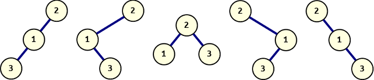
All of these binary trees share a pre-order sequentialisation ([2, 1, 3]). Only one of them is a conforming binary search tree, which is the form we usually mean when we talk about a binary tree, but all of them are valid trees.
A different approach
Clearly, we cannot rely on the ordering of individual values of any individual sequentialisation. The solution to this problem has to come from inherent characteristics of the two different sequences, or more specifically, the differences between them. Let’s go over what we know about each sequentialisation, how they differ, and how we can use those properties to our advantage. [3]
1: Left descent until pre-order matches in-order
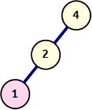
Left descent rule
- The pre-order sequence starts at the root node
- The in-order sequence starts at the furthest left node
This means that at the start, we can read values from the pre-order sequence and expand the tree along a left edge until the current in-order value is reached. The illustration on the right shows how the initial left descent of this tree is constructed from this rule.
2: Move right when pre-order matches in-order
- The pre-order sequence contains nodes along the traced path
- The in-order sequence sweeps the tree from left-to-right horizontally
Whenever the current values from the pre-order and in-order sequences are identical, the next node is to the right of the current node, either further down, or back up along the tree. To account for the case of the next node being further up the tree, we’ll need to maintain a stack of nodes. We’ll add to this stack each time we descend down the left path, allowing us to come back and attach a node on the right.
3: Backtrack and expand to the right
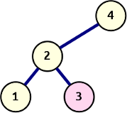
Backtrack and right-expansion
Expanding on that last observation: if we have followed the pre-order sequence to the “left end” and the values from both sequences are now identical, the next value of the in-order sequence will either be …
- … the top value on the stack, which means the algorithm must backtrack to that node and continue to pick from the in-order sequence;
- … not on the stack, and thus a right descendant (though not necessarily an immediate child) of the current node.
This latter situation is similar to the one at the root, with one small difference: the first value from the pre-order sequence is attached to the right of the current node. From there, the tree is expanded along the left edge, using values from the pre-order sequence, until the current in-order value is reached. This could be the very first value that is used to create the node on the right.
At the end of this, pre-order and in-order sequence values are the same, which is a case that’s covered. Once either sequence is completely consumed, construction is finished.
Implementing the algorithm
From these observations and basic rules, we can create a Python implementation that creates a binary tree from pre_order and in_order iterators.
def construct_from_preorder_inorder(pre_order, in_order):
    pre_iter = iter(pre_order)
    root = node = Node(next(pre_iter))
    stack = deque([node])
    right = False

    for ivalue in in_order:
        if stack and ivalue == stack[0].value:
            node = stack.popleft()
            right = True
            continue
        for pvalue in pre_iter:
            if right:
                node.right = node = Node(pvalue)
            else:
                node.left = node = Node(pvalue)
            if right := pvalue == ivalue:
                break
            stack.appendleft(node)
    return root
The setup to this function is pretty similar to our function which constructs a binary search tree from just a pre-order traversal:
- An iterator is retrieved from the pre-order sequence (to support
nextand continued iteration) - A root node is created and also assigned as current
- A stack is created that is used to control backtracking
New in this algorithm is the variable right, which we use to indicate that the next node gets added as a right child, rather than the default left. The in-order sequence is only iterated over in a single continuous loop, so there’s no need to create an explicit iterator for that one.
The main loop is broken up in two branches, similar to the previous example:
- Backtracking: If the in-order value is the same as the current value on the stack, we need to backtrack to that node. We also know the next node will be attached to the right (of that node or one further up the tree), because the in-order sequence makes a left-to-right sweep across the tree.
- Expansion: If we’re not backtracking, we’re descending down to the current in-order value. The first of these steps might be a right step (if we just backtracked), but any additional are left-only. Once we reach the current in-order value, we
breakand setright = True.
There is a little bit of redundancy in setting the right variable during backtracking (rather than just at the end of expansion). This is to cover the case of a tree where the root is also the left-most node. If the in-order sequence is guaranteed to be a list, the initial value for right could be set to node.value == in_order[0] instead.
In conclusion
Sometimes, it only takes a pair of lines of ‘trivial falsehood’ to send you down a rabbit-hole that keeps you engaged days. I figured out my error in comprehension soon enough, but at that point I was already hooked. Looking up the relevant algorithm would have been quicker and easier, and any further questions would have been easy enough to solve with a few keyword searches. However, occasionally, chasing down the rabbit hole and uncovering its secrets can be as instructive as it is entertaining. It is through doing that we learn best.
After this chase, I spent a bit of time looking around for other solutions or papers on the subject, but wasn’t able to find a whole lot (plenty of algorithms of different levels of clarity, but few explanations). What I did find is a 1989 paper from Erkki Mäkinen “Constructing a binary tree from its traversals” which provides a similar algorithm to the one explained above, but with the pre-order sequence in the outer loop. This paper mentions two others, both of which are quoted as less efficient in either time (O(n^2)) or space (unspecified), but remain locked behind a paywall.
Footnotes
| [1] | From the Zen of Python. |
| [2] | Turning expression trees into serialised form has been a recent subject of interest of mine. SQLAlchemy hybrid utils takes SQLALchemy expressions and turns them into a serialised form that can be evaluated against Python objects rather than executed on the database. This allows for a significantly simpler (shorter) way of defining a certain class of hybrid properties. |
| [3] | The process here is far more messy than the distilled results. It’s a lot of trial and error: sheets of paper with numerous graphs scribbled on them and a pile of cut up index cards to simulate different approaches until something works, until something clicks. |
Comments
comments powered by Disqus