Creating a forest from a single seed

Seeing the trees

At this point, before we attempt to create our own forest of binary trees, it’s a good time to look into visualising the trees we plan on making. At its core, a binary tree is a specific type of graph, and there are a ton of tools out there to visualise graphs. One of the more popular open source solutions is the excellent GraphViz. There are various Python packges that provide an interface for it, with pros and cons to all of them, a review of which is well outside the scope of this post. So in short, we’ll be using PyDot, which creates graphs in GraphViz’ Dot format, which we can then have rendered to various image formats.

from collections import deque
from functools import lru_cache
from pydot import Dot, Edge, Node

NODE_STYLE = {
    "fillcolor": "lightyellow",
    "fontname": "ubuntu mono bold",
    "fontsize": 18,
    "penwidth": 2,
    "shape": "circle",
    "style": "filled",
}


def draw(root, name):
    """Renders a tree as PNG using pydot."""
    graph = Dot(nodesep=0.3, ranksep=0.3, bgcolor="#ffffff00")
    graph.set_edge_defaults(color="navy", dir="none", penwidth=4)
    graph.set_node_defaults(**NODE_STYLE)
    graph.add_node(Node(root.value))
    nodes = deque([root])
    while nodes:
        node = nodes.popleft()
        if child := node.left:
            graph.add_node(Node(id(child), label=child.value))
            graph.add_edge(Edge(id(node), id(child)))
            nodes.append(child)
        draw_node_divider(graph, node)
        if child := node.right:
            graph.add_node(Node(id(child), label=child.value))
            graph.add_edge(Edge(id(node), id(child)))
            nodes.append(child)
    graph.write_png(name)


def draw_node_divider(graph, node):
    """Draws a divider to ensure visible single branch direction."""
    target = id(node)
    for _ in range(height(node)):
        parent, target = target, f":{target}"
        graph.add_node(Node(target, label="", style="invis", width=0))
        graph.add_edge(Edge(parent, target, style="invis", weight=5))


@lru_cache
def height(node):
    """Returns the number of ranks below the given node."""
    if node is None:
        return -1
    return 1 + max(height(node.left), height(node.right))

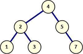
An example binary tree

A binary tree created from a basic Dot graph, with invisible nodes and edges under 4 and 5 to ensure that single child nodes get drawn on the appropriate side.

A few quick remarks on the above code snippet. The draw function sets up a pydot graph and a few basic styles to make it look a little bit nicer. The drawing loop implements a breadth-first-search algorithm, because the order in which the left and right children are added matters, and we need to also add a divider between them (more on that in a moment). For each tree node, its children are added as Dot nodes, and edges are drawn from the parent down the child.

Now, about that divider. GraphViz is pretty good about drawing a node with two children: two diverging lines down to a bubble for each node. However, if there is only a single child, it will draw a line straight down, making it rather difficult to tell a single left child from a single right. To avoid this situation, we add a dummy child tree in the middle. An invisible divider wall to separate left and right, exactly tall enough to reach the bottom of the tree. Increasing its weight parameter above the default ensures that it will become the vertical barrier that all child nodes must diverge away from.

And so, borrowing the simple Node definition from the previous post with an alias, we can now easily create the example tree from the previous post:

left_branch = TreeNode(2, TreeNode(1), TreeNode(3))
right_branch = TreeNode(5, None, TreeNode(7))
example = TreeNode(4, left_branch, right_branch)
draw(example, "example-tree.png")

Insert locations

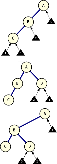
Next-node loci for next value in pre-order sequence for different trees.

Alright, now that we can actually see the different trees we plan on growing, we need to consider how to approach that, and figure out some basic rules. The graphs to the right should help illustrate this a bit further.

All three depth-first search sequentialisations can be reconstructed to trees that fit the description, but the pre-order type makes it particularly easy, given that it starts with the root node and progressively deepens, modulo some occasional backtracking.

For an empty tree, the number of insert loci is trivial: there’s only one, the root node. Once the root node has been put down, the next node can be attached as its left or right child.

If the root node has a left child (and maybe that child has a left child as well, as illustrated), the next node can be a child of any of these nodes. The last inserted node is the tip of that left branch and it can either be a child there, or anywhere within reach of backtracking.

Once the root has a right child, all those possible attachment loci on the left branch disappear: the last inserted node is the root’s right child, and when we backtrack up to there, there are no additional unused branches. We’re left with just the left and right branches of that last node.

However, if that last node was attached somewhere down along the left branch, its path backtracking up to the root would also allow for insertion on the right child branch of the root. This demonstrates that the last inserted node has two attachment loci, and up along its path back to the root, additional loci appear on the right (for every left branch that is tracked back along).

Recursive branching

There is one small problem with the summary statement from the last section: given a leaf node, there is no way to easily determine the parent, because the Node class doesn’t track that, and searching an unordered tree takes linear time. We could of course add a parent attribute, but instead of doing that, let’s see if we we can’t solve it with a slightly more clever approach.

Given that the pre-order sequence describes the nodes in traversal order, we know two important properties of the last-inserted node:

1. It is at the end of a branch (i.e. has no children)
2. It is on a rightmost branch, following left-to-right tree traversal

This means that from the root, we should traverse down until we can descend no further. All the while, we’ll explore right branches before left ones. Further, each time we go left it’s because there’s an unused right branch that we could attach a possible next child to. If we make note of those as we descend, there is no need to backtrack once we reach the last-inserted node!

From this approach, the following recursive construction algorithm follows naturally:

 1
 2
 3
 4
 5
 6
 7
 8
 9
10
11
12
13
14
15
16
17
18
19
20
21
22
23
24
25

def tree_generator(preorder):
    root, *additional = map(Node, preorder)

    def _constructor(root, nodes):
        if not nodes:
            yield root
            return
        cursor = root
        while True:
            while cursor.right is not None:
                cursor = cursor.right
            cursor.right = nodes[0]
            yield from _constructor(root, nodes[1:])
            cursor.right = None
            if cursor.left is None:
                cursor.left = nodes[0]
                yield from _constructor(root, nodes[1:])
                cursor.left = None
                return
            cursor = cursor.left

    return _constructor(root, additional)

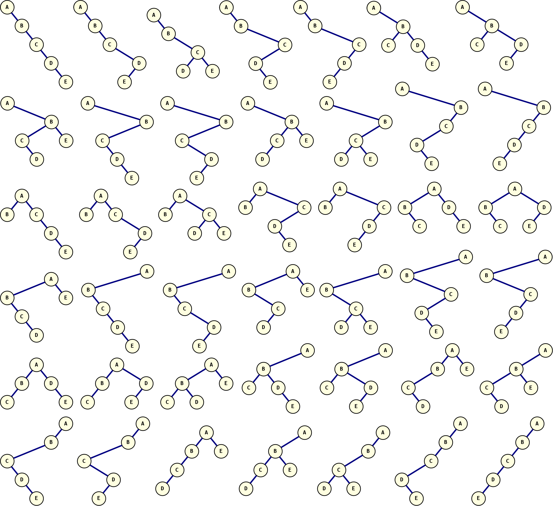
for i, tree in enumerate(tree_generator("ABC")):
    draw(tree, f"tree-abc-{i}")

The code above will draw the five different trees that share the pre-order sequentialisation ABC.

There is one big drawback to the way this generator does its work, which is that there is only a single tree (root node) that gets modified between each iteration. When used in a loop like we do here that’s not a problem, but if you wanted to capture the different trees in a list, you’d end up with a list of 5 references to the same exact tree (in its final configuration).

In an ideal world the tree_generator would return independent trees. This would require some additional function to create a quick copy of the tree, at which point immutable data structures would also be a very nice feature, as it would allow the commonalities between the trees to be safely shared. Building up immutable trees would also remove the need for the “undo” steps on lines 14 and 18. For now though, that’s left as an exercise for the reader.

How big does the forest grow?

Now that we have the means to generate all trees conforming to a given pre-order sequence, one obvious question is “How many trees do we expect to generate for a given sequence length?” If each next node could go anywhere in the tree, the forest would grow at a rate factorial to the size of the trees: a binary tree of size n has exactly n + 1 branching opportunities. That’s a fun property and something of an upper bound, but not quite what we’re looking for.

When discussing this combinatorial question with a coworker, they mentioned the Encyclopedia of Integer Sequences, which has an amazing search function. Putting in the results for the first few forest sizes then points at the Catalan number sequence. This has two leading ones, the first of which is the number of trees that match an empty pre-order sequence. Experimentally, all of these results match up, before they quickly become impractical to count.

The Wikipedia page on Catalan numbers mentions in the introduction that they “occur in various counting problems, often involving recursively defined objects,” and the article goes on to list a large number of examples. One of these examples illustrates differently structured (unlabeled) binary trees, which is close to what we have in our case. We may have values attached but we’re not free to change/swap any of them, so the nodes may as well be unlabeled.

So how many trees of size 6 will be in our forest? The factorial we saw earlier does make an appearance, but it’s tempered by two more. Changing the order of operations a little bit to eliminate parentheses the Catalan number function is factorial(2 * n) // factorial(n + 1) // factorial(n). For n = 6, this results in 12! / 7! / 6! which builds up to 479001600 (12!) and breaks this down to a final 132.

It’s at first surprising to see that this formula results in exact integers, but on closer inspection it’s easy to see how 2n! can be divided by (n+1)! (full overlap of factors). That this result can be divided again by n! is due to the remaining multiplicands (n+1..2n) containing all the factors that comprise 1..n. Working out a few numerical examples on paper makes this really obvious.

A final forest

The only fitting way to end this post is with a forest of our own creation. Below are all the different trees created from the pre-order sequence ABCDE. There’s 42 of them, which feels like a very correct answer: